Here we discuss ElasticSearch Machine Learning. ML is an add-on to ElasticSearch that you can purchase with a standalone installation or pay as part of the monthly Elastic Cloud subscription.
ElasticSearch Machine Learning
The term machine learning has a broad definition. It is a generic term handed over to the laymen as a way of avoiding discussing the specifics of the various models.
To be specific what ElasticSearch ML does is unsupervised learning time series analysis. That means it draws conclusions from a set of data instead of using training a model (i.e., supervised learning) to make predictions, like you would with regression analysis using different techniques, including neural networks, least squares, or support vector machines.
How is this Useful
To see the value of unsupervised learning time series analysis consider the typical approach to cybersecurity or application performance monitoring. That is to assume data follows a normal (gaussian) distribution and then select some threshold that one considers significant when flagging outliers.
This is the familiar bell curve approach. Even if one does not think of it that way, that’s what they are doing. This curve is described by terms the highschool math student should know: mean, variance, and standard deviation. But that is not machine learning.
Not Better than Guessing
Typically someone doing application monitoring or cybersecurity flags an event when it lies at either end of the curve, which is where the probability of such an event is low. That’s usually referred to as some multiple of σ (sigma), where sigma is a multiple of standard deviations, where the probability of an event lying there is very low.
You could also with derision call this approach guessing.
The threshold approach is flawed, because it leads to false positives. That causes analysts to spend time tracking down events that are not truly statistically significant.
For example, with cybersecurity, just because someone is sending data to a particular IP address more now than before does not mean that event is out of bounds. They need to consider the cyclical nature of events and look at current events in light of what has come before them. It could be this happens every month and is normal. A clever algorithm can do that by, for example, applying a least squares method and looking to minimize the error (i.e., the difference between what is observed and what is expected), against a shifting subset of data. This is how ElasticSearch does it. And they apply several algorithms, not just least squares.
How to use ElasticSearch to do Machine Learning
Here we show how to use the tool. In another blog post we will explain some of the logic and algorithms behind it. But the tool is supposed to make it not necessary to understand all of that. Still, you should so you can trust what it is telling you.
We are going to draw from this video by ElasticSearch and slow it down to single steps to make it simpler to understand.
For data we will use the New York City taxi cab dataset that you can download from Kaggle here. The data gives us pick up and drop off times and locations for NYC cabs over a period of a few years. We want to see when traffic falls off or increases in such a way that is an abnormality, like a taxi strike or snowstorm.
There are some limits with loading this data in the Kibana ML screen, which is a feature with ES ML. You can only load 100 MB of data at a time. The taxi cab data is much larger than that. It includes a test and train dataset. Since we are not training a model with unsupervised learning, we will just pick one of them. And since we need to limit it to 100 mb we will split the 200 mb data file like this and just pick one 90MB dataset.
unzip train.zip
split -b 90000000 train.csv
Also note that ElasticSearch tends to freeze up when you load data like this, unless you have a large cluster. But it still loads the data. So once it looks like it has finished loading, meaning the screen no longer updates, just click out of it and to go to Index management to see how many records are in the new index. It should be about 100,000 for each 90MB of data.
Upload the Data into the Machine Learning Screens
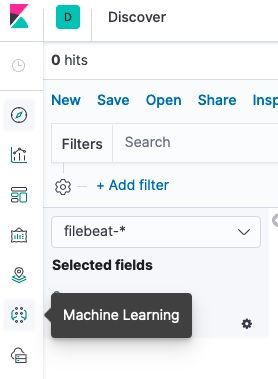
Open Kibana and click on the Machine Learning icon. You will have that icon even if you don’t have a trial or paid license. But what will be missing is the Anomaly Detection, job creation, and other screens. So ElasticSearch will guide you through signing up for a trial.
From the Data Visualizer select Import a file and import one of the files you split from train.csv. Or if you loaded the data a different way you can use the Select an Index Pattern option.
ElasticSearch will show you the first 1,000 rows and then make some quick record counts.

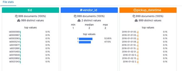
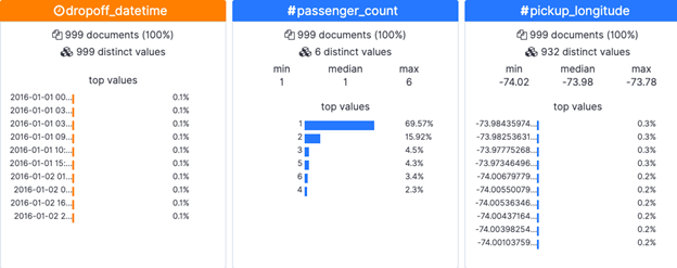
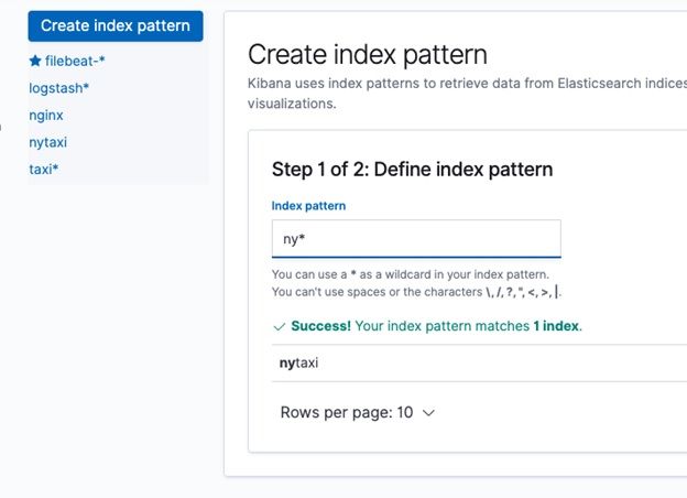
Then click Import at the bottom of the screen. Give it a name for the Index Pattern name, like ny*.
Anomaly Detection
Now we get to the interesting part. We want ElasticSearch to look at this time series data. Pick the Single Metric option.
Then we have to create a job. ElasticSearch will run an aggregation query in the background. We tell it to sum passenger_count over time. (If the drop down box does not work just copy and paste the field name.)
We use this aggregation to observe when there is a drop off or spike in passengers that lies outside the normal range and that takes into consideration the normal rise and fall of passenger count over time.
Click the button Use Full Range of Data, so it will pick all the data available and not the date interval you manually put. You can change the bucket option to 10m.
Then the screen will fill out like this:
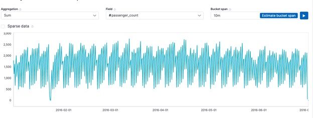
Then click Create Job. It starts running its algorithms and updating the display with vertical colored lines as it completes its logic.
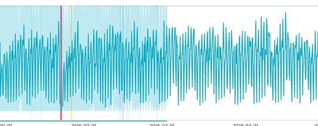
View the Anomaly Detection Results
When it is done click View Results.
We will explain in another post exactly what calculations it has done, after all you should not trust an ML model without having some understanding of how it drew its conclusions.
But you can think of it like this. Taxi rides go up and down during the week versus the weekend and rush hour versus not. If you were working with sales data you would call that trends or seasonality. So if you used a gaussian (normal) distribution against that it would be wrong, as the mean and variance would be over the whole set including the high and low points. So the improved algorithm slides along making multiple normal curves (and other frequency distributions) against subsets of the data to eliminate this up and down pattern.
This produces the results below. The light blue area is the shifting probability distribution function. The red area is where you can see is the anomaly, the point where the plot has gone outside the curve. It’s also the point where we have run out of data. It has flagged that as an outlier by calculating an anomaly score, a point we will cover in the next post.


